October has been the most volatile month for stocks on average over the past 87 years. Is this result purely due to chance, or should we take it seriously and expect it to continue into the future? To answer this, we assess the statistical significance of the extreme October volatility values, and we demonstrate that correctly accounting for multiplicity is crucial to properly interpreting the results.

Seasonal effects in stock markets is a topic of ongoing discussion within the industry, with some believing in an October effect, a January effect, and the old adage “sell in May and go away”. These maxims often seem to be founded upon anecdotal evidence, but a prudent investor would need something more statistically rigorous. As a reasonable first step in investigating seasonality, we examine if market volatility is significantly high or low for any calendar month.

We use 87 years of S&P 500 daily returns as a proxy for long-term market dynamics. For each year of data, annualised volatilities are calculated for each month. These volatilities are then ranked from 1 to 12 (lowest to highest volatility) in each year, and an average rank is then calculated over the 87 years. The results of this analysis are shown in Figure 1.

Figure 1: Mean rank for each month by S&P volatility

Calendar months were ranked by volatility of the S&P 500, for every year from 1928 to 2014. The chart shows the mean rank for each month. October and December have the highest and lowest volatilities respectively.

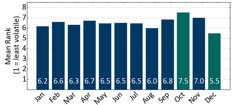
October has clearly been more volatile than other months, and December has been less volatile. Both of these are equally extreme, in terms of their absolute deviation from the expected value of 6.5, and it is natural for someone viewing these results to highlight them as an important feature of the data.

But before getting carried away and speculating over the cause of the extreme October volatility values, we should establish how significant this observation is [1]. If it is statistically significant then we might expect the feature to repeat in the future, and if it isn’t significant then there is a good chance that no seasonal effects are actually present.

It is important to note that before we analysed the data, we would have been interested in the most extreme point in Figure 1 regardless of the month it fell in, and whether it was high or low. Therefore, we have in fact tested all the months of the year simultaneously, and are faced with a multiplicity issue which requires a bit of extra care.

Incorporating multiplicity

Statisticians often work with “p-values” when analysing features in data and comparing hypotheses. A p-value quantifies the probability of seeing a result at least as extreme as the one observed in the case of the null-hypothesis being true. For a result to be interesting, it should have a low p-value, but the exact threshold used to define something as significant is a subjective decision.

For our analysis we will set a significance level of 0.05. This means there should be only a 5% chance of accidentally classifying a result as significant if the null hypothesis was true. For this work, the null hypothesis is that all months are expected to have the same volatility because no seasonal effects are present.

Now consider what happens if you apply this logic to 12 tests, one for each calendar month. The probability of observing at least one month with an apparently significant volatility, in the case of the null hypothesis being true, is given by [2]:

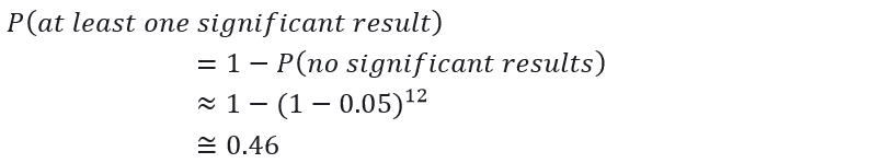
We see that when multiplicity is not accounted for, there is a 46% chance of observing an apparently significant result.

How should multiplicity be incorporated when determining if any month’s volatility is statistically significant? To resolve this we must understand the difference between asking the following two questions:

• Question 1: “How likely is it that October would appear this extreme by chance?”
• Question 2: “How likely is it that any month would appear this extreme by chance?”

This difference is illustrated in Figure 2. To make these plots, we calculated 1,000 sets of 12 average volatility ranks, using 87 years of simulated data for each set. No seasonal effects were present in the simulated data. The absolute deviation of the volatility ranks from the expected value of 6.5 were recorded.

Figure 2. Probability distributions generated by simulations which assume there is no seasonality in market volatility

The distributions are shown for the absolute deviation of mean volatility rank from the expected value of 6.5. The left plots show the result for any month. The right plots are for the most extreme month. The dashed red lines indicate 0.05 significance level thresholds.

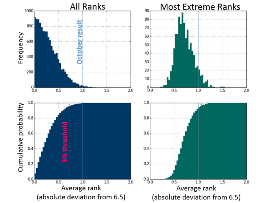
The left hand probability and cumulative distributions were made using all 12,000 absolute deviations. This is the distribution that would be used to answer Question 1, and it would appear that an interesting result (at the 5% level for a one-tailed test of significance) is one with an absolute deviation of at least 0.73. This makes the October result (1.0 absolute deviation) appear significant, with only a 0.7% chance of observing a more extreme value in the case of the null hypothesis being true.

But this significance threshold is based on comparing a single month to the distribution of all absolute deviations, whereas we effectively compared 12 when we selected the most extreme value.

To account for multiplicity and to know if the October result is truly significant we need to compare it with the distribution of the most extreme volatility ranks from each of the 1,000 simulated sets. To do this, for each simulation we record just the largest absolute deviation value, and this distribution is shown on the right hand side of Figure 2.

We see that incorporating multiplicity makes the threshold of significance more conservative. To be considered a significant result, an absolute deviation would actually need to be at least 1.1. This makes October’s volatility value no longer significant, with an 8% chance of observing a more extreme value of average volatility rank if the null hypothesis is true.

Conclusion

In our simple test we failed to find sufficient evidence to support the existence of seasonal volatility in historical returns for the S&P 500.

At first glance October appears to have extremely high volatility, driven by crises such as those of 1929, 1987, and 2008. While we cannot rule out that S&P volatility will be driven by some seasonal effects in the future, we can quantify the probability of seeing results as extreme as ours in data that is not seasonal, and it stands at 8%.

Had we not incorporated multiplicity into our analysis, then this probability would look far more interesting, at 0.7%. This straightforward seasonality example highlights the importance of using rigorous statistics in the world of investment management.

This article contains simulated or hypothetical performance results that have certain inherent limitations. Unlike the results shown in an actual performance record, these results do not represent actual trading. Also, because these trades have not actually been executed, these results may have under- or over-compensated for the impact, if any, of certain market factors, such as lack of liquidity and cannot completely account for the impact of financial risk in actual trading. There are numerous other factors related to the markets in general or to the implementation of any specific trading program which cannot be fully accounted for in the preparation of hypothetical performance results and all of which can adversely affect actual trading results. Simulated or hypothetical trading programs in general are also subject to the fact that they are designed with the benefit of hindsight. No representation is being made that any investment will or is likely to achieve profits or losses similar to those being shown.

This article contains information sourced from S&P Dow Jones Indices LLC, its affiliates and third party licensors (“S&P). S&P® is a registered trademark of Standard & Poor’s Financial Services LLC and Dow Jones® is a registered trademark of Dow Jones Trademark Holdings LLC. S&P make no representation, warranty or condition, express or implied, as to the ability of the index to accurately represent the asset class or market sector that it purports to represent and S&P shall have no liability for any errors, omissions or interruptions of any index or data. S&P does not sponsor, endorse or promote any Product mentioned in this material.

Using a rank methodology induces a slight dependence between results, but this does not affect the general implication of the argument.