16 March 2023 | 5 min read
Different approaches to quantitative investing

Originally published on the CAIA Portfolio for the Future blog on 16 March 2023.
Quantitative investment management resembles the natural sciences, in that it attempts to understand phenomena through empirical analysis of data. It is common for researchers to use techniques developed for scientific analysis to predict market movements and create novel trading strategies. We assess which methods are most pertinent for different trading strategies and discuss the challenges associated with using techniques such as machine learning.
Experimental vs Observational Science
One aspect of the scientific process that is significant for quantitative investment management is the distinction between experimental and observational investigations. Experiments can be repeated many times to generate large datasets of comparable results. To take an example from physics: a particle accelerator smashes protons together to see how often a Higgs particle is produced from the resulting debris. If more data are needed to measure more precisely the likelihood of Higgs production, the process can be repeated (budget allowing) until the desired level of precision is reached. This may generate billions or trillions of data points.
Contrast this experimental approach with an astronomer studying the gravitational waves produced by colliding black holes. The astronomer examines as many actual collisions as possible, and theorises about the precise details of the resulting waves. There is no way to create a large number of comparable pairs of black holes and set them in motion to see what occurs. Moreover, the relative scarcity of black holes makes it likely that the set chosen will not be a representative sample and thus contain biases. In this observational approach, astronomers must take the universe as they find it, try to correct biases in their data, and draw conclusions from the available information.
However, experiment and observation are not a rigid dichotomy but rather two directions of travel on a continuous scale. The more it is possible to control and repeat the process of creating relevant data, the further one can move towards the experimental end of the scale. Going in the other direction, datasets become smaller in size and more prone to various forms of bias, with signals often harder to distinguish from noise.
The distinction between experimental and observational research extends to finance. For example, an execution algorithm can be tested experimentally by applying it to additional trades. Yet a theory about stock-market crashes can be studied only observationally, since the only data comes from crashes that have already taken place, with widely varying circumstances in each case. More crashes cannot be generated on demand!
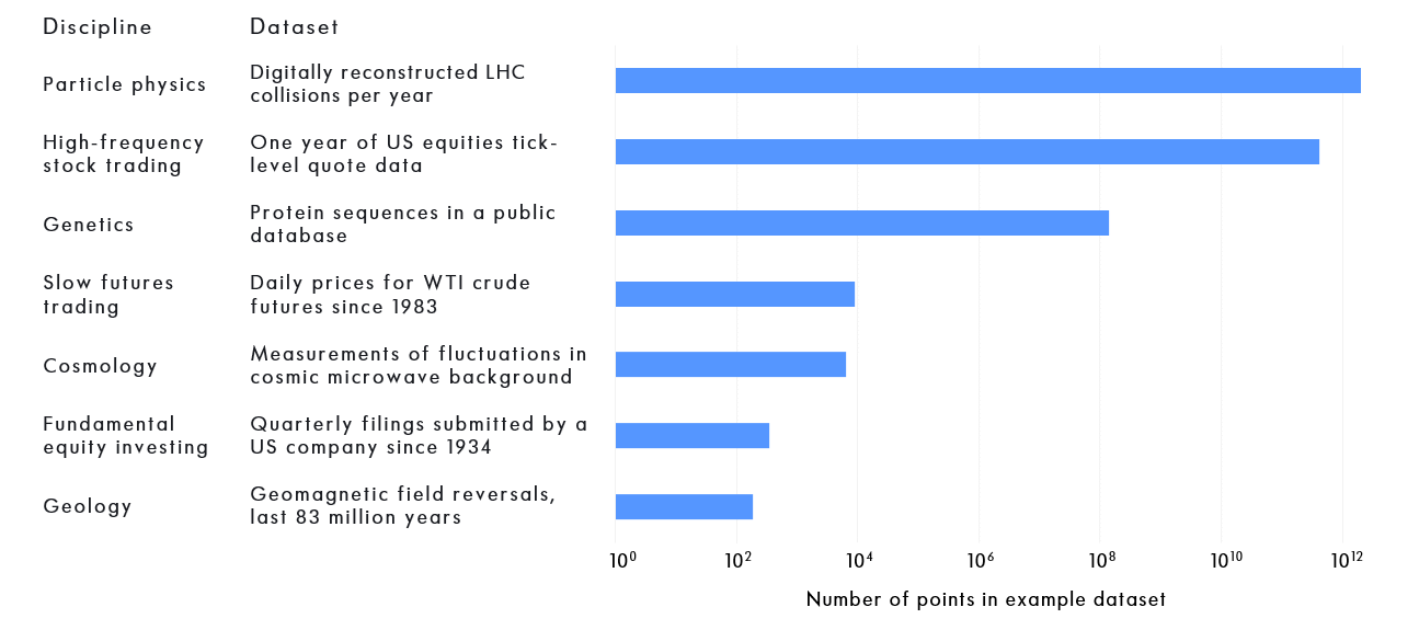
The datasets found in finance span a similar range in size to those in science, as we show in the following figure. At one extreme, long-term fundamental investors must often cope with only a few hundred data points, since most listed companies issue financial statements only quarterly. At the other, high-frequency traders process prices stamped to the nanosecond, with the resulting datasets comparable in size to those used in particle physics.
Comparison Between the Sizes of Example Financial and Scientific Datasets

As suggested by the above figure, the different amounts of data available to high-frequency and low-frequency traders determine their positions on the experiment-observation scale. Both types of trader invest in the same markets, but high-frequency traders use the vast amount of data that is available at shorter timescales. This enables them to operate experimentally, because they have more data against which to assess their ideas.
Faster trading signals are more suited to experiments for another, more practical reason: they often have higher expected Sharpe ratios, which means that they can be judged more quickly by their out-of-sample performance.
If, for example, a signal with a supposed Sharpe ratio of 2 or more has produced losses after a few months, it is likely that something is wrong – perhaps the idea has been widely discovered and “arbitraged out”. The signal can then be switched off, and a new experiment started. By contrast, a strategy with an estimated Sharpe ratio of 0.5 could be down for more than a year, but it would not be rational to stop trading the strategy due to performance alone. This is because a multi-year loss is consistent with the long-term expected statistical distribution for that level of Sharpe ratio.
Experiment and observation thus represent two different approaches to quantitative investment. The experimental method involves looking for faster strategies with higher Sharpe ratios. Individually, these strategies will have limited capacity because of the transaction costs incurred by their relatively frequent trades. The aim, however, is to build a large portfolio by combining lots of fast signals.
The alternative approach is to seek out signals that have higher capacity, and generally lower Sharpe ratios. Fewer such signals are needed to build a large portfolio, provided they have low correlation to one another.
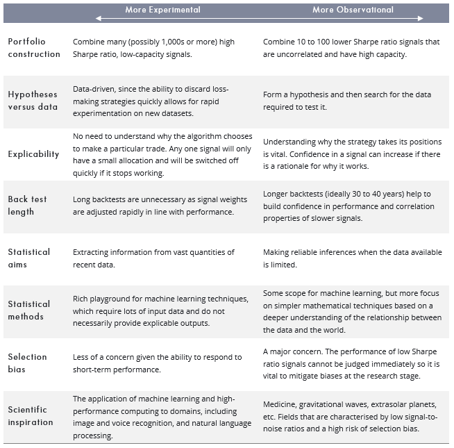
As in the scientific arena, experiment versus observation is a spectrum, not a binary choice. It is, nevertheless, a useful framework for understanding the alternative methods used by different quantitative investment managers. We summarise some of the main differences in the following table.

Use of Machine Learning
The rapid recent increase in the amount of data available in just about every sphere has created new possibilities for predictive modelling.
For example, a traditional equity analyst might read every report produced by or about the companies they cover, and may in the past have known every relevant fact or figure about a specific company when making an earnings forecast. The data used in an earnings forecast today, however, could include satellite imagery, credit card spending information, logistical details of every product on every truck, and much more besides.
It would be impractical for a person or group of people to pay as close attention as in the past to this massively increased amount of data. But this apparent problem is a great opportunity to apply a collection of statistical techniques known colloquially as “machine learning”. From recognising the content of images to making targeted recommendations on retailers’ websites, the success of these methods has been extraordinary. But they have one vital requirement: a lot of input data.
Hence the applicability of machine learning to faster trading strategies: the volume of short-term price information generates large amounts of data. With slower trading systems, the comparatively limited information content of small, noisy datasets is a less appropriate input for machine-learning models. In such cases, it is more useful to work on drawing reliable conclusions from the data, and to concentrate on interpretability and simplicity rather than applying unnecessarily complex algorithms.
That said, at Winton we have also found machine learning methods to be useful for slower trading strategies. This is because our data requirements can often be significant, particularly if we want to perform a lengthy backtest. By way of example, consider a trading strategy that analyses the text of quarterly company reports. To perform a 40-year backtest on the largest 1,000 US companies, we would need to analyse 160,000 reports. And any change to algorithms using the data would require all the reports to be analysed afresh. This task is beyond a group of individuals. Machine learning methods are appropriate instead.
The Danger of Selection Bias
At Winton, our research is often hypothesis-driven. A researcher will start with an idea about the world, and then search for data to test whether it is correct. When it comes to creating a trading signal from the idea, the aims are low correlation to existing strategies and a positive Sharpe ratio.
These goals may sound modest. Yet finding just 16 uncorrelated signals, each with a Sharpe ratio of 0.5, would result in a portfolio with a Sharpe ratio of 2 – a far less modest ambition!
This is difficult to achieve in practice, however. While it is easy to create a backtest of a trading signal with a positive Sharpe ratio, it is extremely hard to be sure that the Sharpe ratio will remain positive in future. Statistical estimation error is one issue. A much more pernicious problem is selection bias.
To grasp how selection bias operates, imagine coming up with 100 random trading signals, which by definition have no insight or power to predict market movements. Nevertheless, their performance in a backtest will not be precisely zero, but will form a distribution, and some of the signals will seem to have Sharpe ratios of 0.3 or higher. If we pick only those with positive historical performance, while discarding the others, we will have created a portfolio with an attractive backtest that in reality has a Sharpe ratio of zero, or less, after including transaction costs.
This is a stylised example, but unfortunately the reality of research can be all too similar. Researchers test lots of ideas, and although they are not generated randomly, we do not know in advance whether they work or not. Even if the ideas are good on average, the best backtests will be partly the result of the idea working, and partly luck, so the true Sharpe ratio is likely to be overestimated.
Moreover, the selection bias arising from picking the ideas with the best backtests is deeply ingrained in many organisational cultures. Employees want to show their managers only their best results. When something works less well, it is easy to file it away and move on to an idea that looks more promising, or to adjust the parameters of the model until it does work. Even when researchers are aware this is happening, they often fashion subsequent explanations for why the original idea would have failed, and so exclude it from the list of ideas they have tried.
A seminal 2005 paper with the dramatic title “Why Most Published Research Findings Are False” widely publicised the effect of selection bias in academia, where the selection is often at the point of publication. Journals are more likely to print papers that report significant results than those that do not. This has resulted in the so-called “replication crisis”, where researchers have been unable to reproduce the results of earlier work.
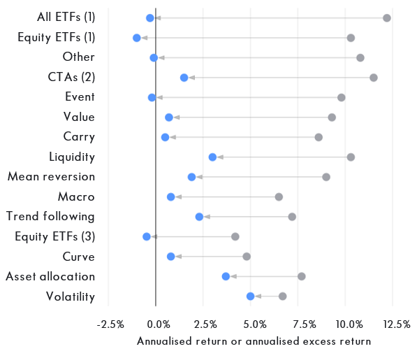
A parallel in investment management is the disparity between the backtest and live performance. We have shown previously the tendency for trend-following products to underperform their backtests after launch. A meta-analysis drawing data from various sources shows that the problem appears across the investment landscape.
Various Studies on the Performance of Investment Strategies Prior to and After Their Launch

As indicated above, the problem of selection bias is not purely technical. It can appear even if all researchers carry out their work to an exemplary standard. The problem is rather with the framework under which the research is organised. The necessity of addressing the issue at an organisational level was discussed in a 2018 paper in the context of machine learning applications in quantitative finance.
Conclusions
Quantitative investment managers operate across a spectrum. One end can broadly be characterised as closer to trading, usually involving higher-frequency strategies; a more experimental approach to implementing new systems; a focus on higher Sharpe ratios and lower capacities; a requirement for large (often intraday) datasets, and an attendant interest in machine learning. The other end is closer to investment, with generally slower systems with lower transaction costs; an approach that is necessarily more observational; sub-strategies with lower Sharpe ratios but capable of managing more capital; and a requisite appreciation of the subtleties of dealing with small amounts of data and finding weak signals in noisy datasets.
Amid the fervent hype, big data and machine learning do offer opportunities for investment managers pursuing slower trading strategies. But more often researchers face the problem of making inferences from relatively small amounts of data. In such cases, care must be taken to extract reliable information.


